8. Making plots

🎯 GOALS

Visualizing ERP effects using time course plots and scalp topography plots.

8.1 Time course

Load required packages:
- ggplot2 for plotting
- dplyr and tidyr for data wrangling

library(here)
library(ggplot2)
library(dplyr)
library(tidyr)
library(eegUtils)

Load preprocessed epochs from a single ERP CORE participant:

bids_dir <- here("data/n170")
deriv_dir <- here(bids_dir, "derivatives/eegUtils/sub-001/eeg")
epoch_file <- here(deriv_dir, "sub-001_task-N170_desc-corrected_eeg.rds")
dat_epo <- readRDS(epoch_file)

Create a time course plot:
- x-axis: Time
- y-axis: ERP amplitude (one electrode or ROI average)
- Colors: Average ERP wave forms in different conditions

plot_timecourse(dat_epo, electrode = "PO7", colour = "epoch_labels")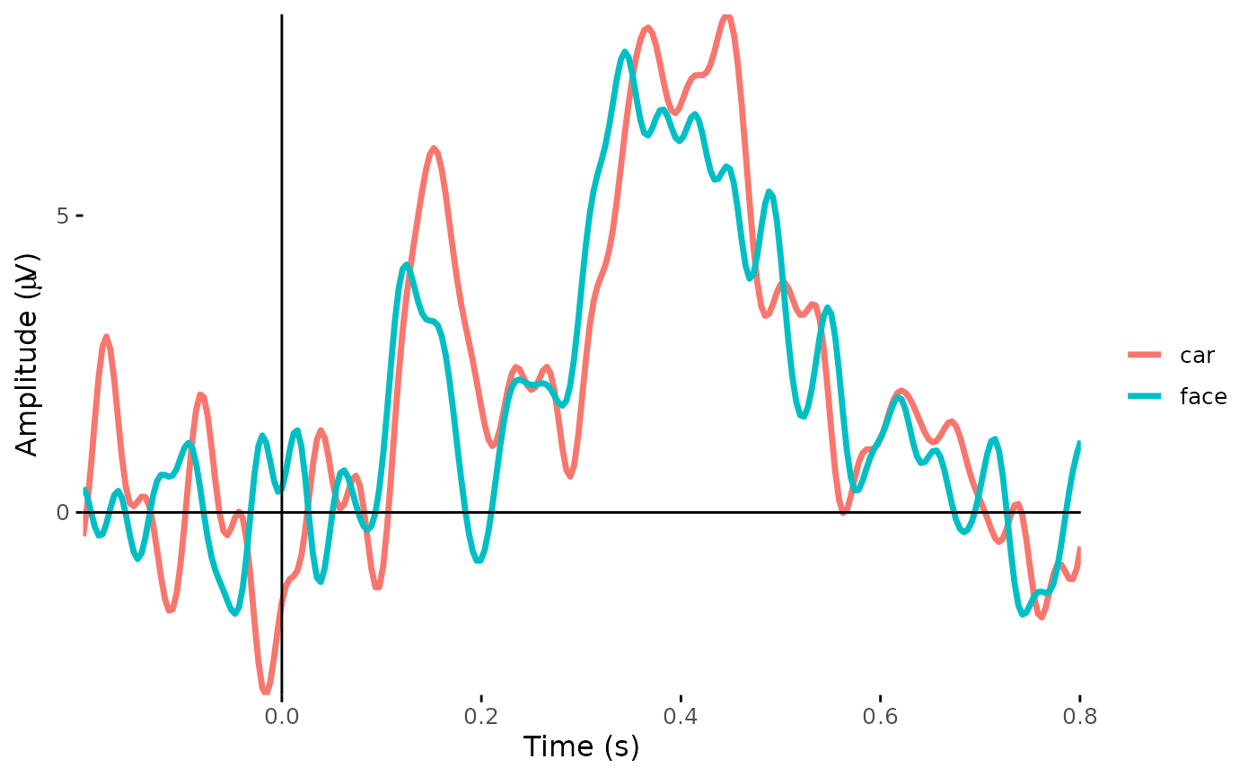

Add annotations for the plotted time window and electrode of interest:

tmin <- 0.15
tmax <- 0.2

plot_timecourse(dat_epo, electrode = "PO7", colour = "epoch_labels") +
  annotate("rect", xmin = tmin, xmax = tmax, ymin = -Inf, ymax = Inf, alpha = 0.2) +
  annotate("text", x = 0.7, y = 8, label = "Electrode PO8")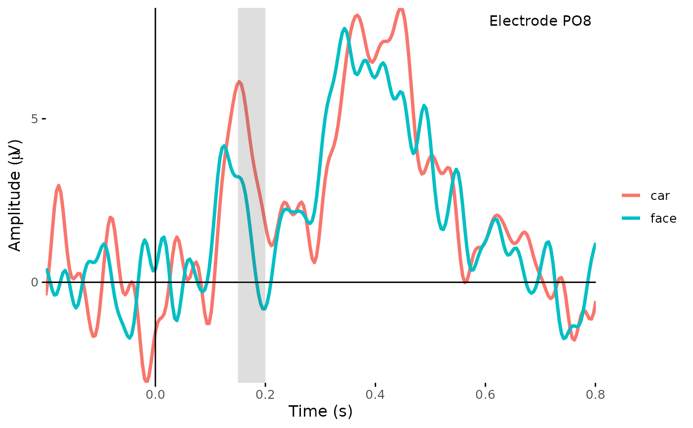

Plot all electrodes:

erp_scalp(dat_epo, colour = "epoch_labels", size = 0.6)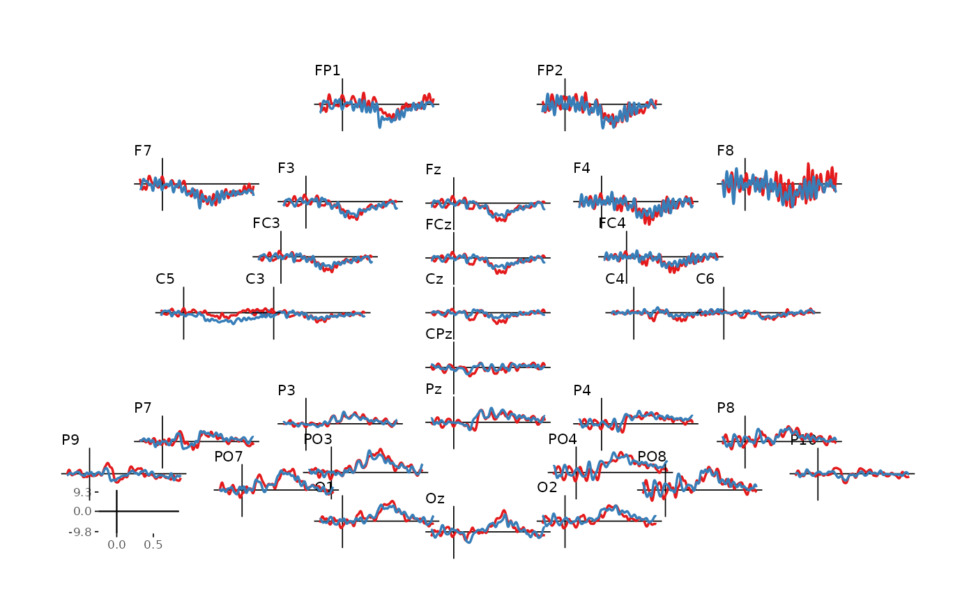

8.2 Scalp topography

Scalp topography shows the distribution of voltages on the scalp
Either for a single condition or (more typically) for the difference between conditions
Requires some wrangling of the data:
- Goal: a data frame with a column of electrode names and a vector of amplitudes
- Using tidyverse style here (see the note in Vignette 1, Section 1.4)

dat_epo %>%
  as.data.frame() %>%
  filter(time >= tmin & time < tmax) %>%
  select(-c(time, epoch, participant_id, recording, event_type)) %>%
  pivot_longer(-epoch_labels, names_to = "electrode", values_to = "amplitude") %>%
  group_by(electrode, epoch_labels) %>%
  summarize(amplitude = mean(amplitude), .groups = "drop") %>%
  group_split(epoch_labels) -> dats_topo

head(dats_topo[[1]])

## # A tibble: 6 × 3
##   electrode epoch_labels amplitude
##   <chr>     <chr>            <dbl>
## 1 C3        car             -1.00 
## 2 C4        car             -2.18 
## 3 C5        car              0.291
## 4 C6        car             -1.73 
## 5 CPz       car             -2.23 
## 6 Cz        car             -2.21

head(dats_topo[[2]])

## # A tibble: 6 × 3
##   electrode epoch_labels amplitude
##   <chr>     <chr>            <dbl>
## 1 C3        face            0.0955
## 2 C4        face            0.417 
## 3 C5        face           -1.86  
## 4 C6        face           -0.0356
## 5 CPz       face            0.0628
## 6 Cz        face            0.615

Create a new data frame that has the difference between face amplitudes and car amplitudes:

dat_topo <- data.frame(
  electrode = dats_topo[[1]]$electrode,
  amplitude = dats_topo[[2]]$amplitude - dats_topo[[1]]$amplitude
)
head(dat_topo)

##   electrode amplitude
## 1        C3  1.099734
## 2        C4  2.595016
## 3        C5 -2.147613
## 4        C6  1.692896
## 5       CPz  2.290653
## 6        Cz  2.822351

Create the topographic plot with eegUtils:

topoplot(dat_topo, limits = c(-6.0, 6.0))

2023-01-03

8.1 Time course

8.2 Scalp topography