2. Preprocessing#
Preprocessing is the first step in EEG data analysis. It usually involves a series of steps aimed at removing non-brain-related noise and artifacts from the data. Unlike the following steps (e.g., epoching and averaging), it leaves the data in a continuous format (EEG channels × timepoints).
Goals
Loading raw EEG data
Plotting the raw data
Filtering the data to remove low and high frequency noise
Correcting eye artifacts using independent component analysis (ICA)
Re-referencing the data to an average reference
2.1. Load Python modules#
We will use the following Python modules:
MNE-Python for EEG data analysis (Gramfort et al, 2013)
hu-neuro-pipeline for downloading example data
Note that on Google Colab, you will need to install these modules first. You can uncomment and run the following cell to do so.
# %pip install mne hu-neuro-pipeline
from mne import set_bipolar_reference
from mne.io import read_raw
from mne.preprocessing import ICA
from pipeline.datasets import get_erpcore
2.2. Download example data#
We’ll use data from the ERP CORE dataset (Kappenman et al, 2021). This dataset contains EEG data from 40 participants and 6 different experiments. Each experiment was designed to elicit one or two commonly studied ERP components.

Fig. 2.1 The six different ERP CORE experiments. Source: Kappenman et al (2021)#
In this example, we’ll use the data from the fourth participant in the face perception (N170) experiment.
files_dict = get_erpcore('N170', participants='sub-004', path='data')
files_dict
Downloading file 'erpcore/N170/README.txt' from 'https://files.de-1.osf.io/v1/resources/pfde9/providers/osfstorage//612e8fb3af610c00b9dff048' to '/home/runner/work/intro-to-eeg/intro-to-eeg/ipynb/data'.
Downloading file 'erpcore/N170/task-N170_events.json' from 'https://files.de-1.osf.io/v1/resources/pfde9/providers/osfstorage//60077b01ba010908a78927da' to '/home/runner/work/intro-to-eeg/intro-to-eeg/ipynb/data'.
Downloading file 'erpcore/N170/participants.tsv' from 'https://files.de-1.osf.io/v1/resources/pfde9/providers/osfstorage//60061136df7ff00036478ff8' to '/home/runner/work/intro-to-eeg/intro-to-eeg/ipynb/data'.
Downloading file 'erpcore/N170/participants.json' from 'https://files.de-1.osf.io/v1/resources/pfde9/providers/osfstorage//60061134df7ff00036478fed' to '/home/runner/work/intro-to-eeg/intro-to-eeg/ipynb/data'.
Downloading file 'erpcore/N170/dataset_description.json' from 'https://files.de-1.osf.io/v1/resources/pfde9/providers/osfstorage//60061132df7ff000314746ab' to '/home/runner/work/intro-to-eeg/intro-to-eeg/ipynb/data'.
Downloading file 'erpcore/N170/LICENSE' from 'https://files.de-1.osf.io/v1/resources/pfde9/providers/osfstorage//6006112bba010907d18928e0' to '/home/runner/work/intro-to-eeg/intro-to-eeg/ipynb/data'.
Downloading file 'erpcore/N170/CHANGES' from 'https://files.de-1.osf.io/v1/resources/pfde9/providers/osfstorage//60061128d77bf1000c677b6f' to '/home/runner/work/intro-to-eeg/intro-to-eeg/ipynb/data'.
Downloading file 'erpcore/N170/sub-004/eeg/sub-004_task-N170_events.tsv' from 'https://files.de-1.osf.io/v1/resources/pfde9/providers/osfstorage//60075c87ba01090877890ad5' to '/home/runner/work/intro-to-eeg/intro-to-eeg/ipynb/data'.
Downloading file 'erpcore/N170/sub-004/eeg/sub-004_task-N170_coordsystem.json' from 'https://files.de-1.osf.io/v1/resources/pfde9/providers/osfstorage//61021546c7a976029b9e5be8' to '/home/runner/work/intro-to-eeg/intro-to-eeg/ipynb/data'.
Downloading file 'erpcore/N170/sub-004/eeg/sub-004_task-N170_electrodes.tsv' from 'https://files.de-1.osf.io/v1/resources/pfde9/providers/osfstorage//61021543c7a976029a9e200c' to '/home/runner/work/intro-to-eeg/intro-to-eeg/ipynb/data'.
Downloading file 'erpcore/N170/sub-004/eeg/sub-004_task-N170_eeg.set' from 'https://files.de-1.osf.io/v1/resources/pfde9/providers/osfstorage//60075c8586541a090014bc12' to '/home/runner/work/intro-to-eeg/intro-to-eeg/ipynb/data'.
Downloading file 'erpcore/N170/sub-004/eeg/sub-004_task-N170_channels.tsv' from 'https://files.de-1.osf.io/v1/resources/pfde9/providers/osfstorage//60075c77ba01090877890ac5' to '/home/runner/work/intro-to-eeg/intro-to-eeg/ipynb/data'.
Downloading file 'erpcore/N170/sub-004/eeg/sub-004_task-N170_eeg.fdt' from 'https://files.de-1.osf.io/v1/resources/pfde9/providers/osfstorage//60075c7f86541a08f914ab5d' to '/home/runner/work/intro-to-eeg/intro-to-eeg/ipynb/data'.
Downloading file 'erpcore/N170/sub-004/eeg/sub-004_task-N170_eeg.json' from 'https://files.de-1.osf.io/v1/resources/pfde9/providers/osfstorage//60075c81e80d3708caa5832c' to '/home/runner/work/intro-to-eeg/intro-to-eeg/ipynb/data'.
{'log_files': ['/home/runner/work/intro-to-eeg/intro-to-eeg/ipynb/data/erpcore/N170/sub-004/eeg/sub-004_task-N170_events.tsv'],
 'raw_files': ['/home/runner/work/intro-to-eeg/intro-to-eeg/ipynb/data/erpcore/N170/sub-004/eeg/sub-004_task-N170_eeg.set']}
2.3. Load raw data#
We read the actual EEG data files (eeg.set/eeg.fdt) into MNE-Python.
The result is a Raw object, which contains the continuous EEG data and some metadata.
raw_file = files_dict['raw_files'][0]
raw = read_raw(raw_file, preload=True)
raw
Reading /home/runner/work/intro-to-eeg/intro-to-eeg/ipynb/data/erpcore/N170/sub-004/eeg/sub-004_task-N170_eeg.fdt
Reading 0 ... 649215  =      0.000 ...   633.999 secs...
General
| Measurement date | Unknown |
|---|---|
| Experimenter | Unknown |
| Participant | Unknown |
Channels
| Digitized points | 33 points |
|---|---|
| Good channels | 33 EEG |
| Bad channels | None |
| EOG channels | Not available |
| ECG channels | Not available |
Data
| Sampling frequency | 1024.00 Hz |
|---|---|
| Highpass | 0.00 Hz |
| Lowpass | 512.00 Hz |
| Filenames | sub-004_task-N170_eeg.fdt |
| Duration | 00:10:34 (HH:MM:SS) |
We can access the actual data array (a Numpy array) using the get_data() method.
raw.get_data()
array([[-0.01593189, -0.0159683 , -0.01600371, ..., -0.01595349,
        -0.01595786, -0.01596058],
       [-0.03090565, -0.03089662, -0.03088733, ..., -0.03030712,
        -0.03030746, -0.03030712],
       [ 0.00585654,  0.00586507,  0.00585632, ...,  0.0053501 ,
         0.00534794,  0.00534897],
       ...,
       [ 0.01395562,  0.01396296,  0.01395765, ...,  0.0130488 ,
         0.01304721,  0.0130503 ],
       [-0.00940747, -0.00941859, -0.00942844, ..., -0.00855003,
        -0.00854672, -0.00854356],
       [-0.00327154, -0.00327973, -0.00327407, ..., -0.0036367 ,
        -0.00363201, -0.00362738]])
Let’s check the size (number of dimensions and their length) of this array:
raw.get_data().shape
(33, 649216)
We see that it has two dimensions (EEG channels × timepoints).
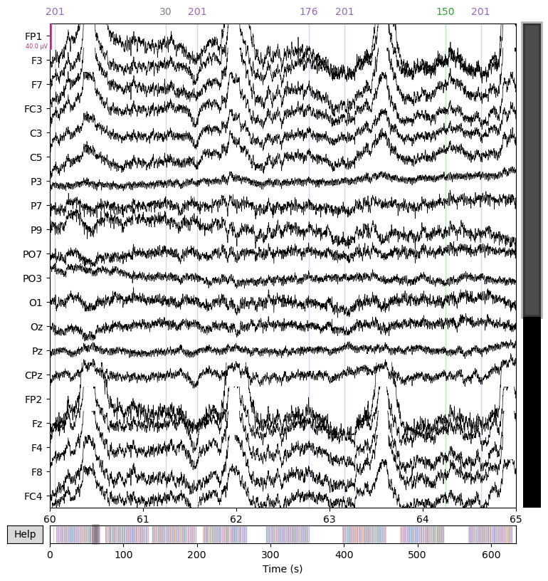
2.4. Plot raw data#
We can plot the raw data using the plot() method.
We specify which time segment of the data to plot using the start and duration arguments.
Here we plot 5 seconds of data, starting at 60 seconds.
_ = raw.plot(start=60.0, duration=5.0)
Using matplotlib as 2D backend.
2.5. Add channel information#
Right now, MNE thinks that all channels are EEG channels.
However, we know that some of them are actually EOG channels that record eye movements and blinks.
We’ll use these to create new “virtual” EOG channels that pick up strong eye signals (vertical EOG [VEOG] = difference between above and below the eyes; horizontal EOG [HEOG] = difference between left and right side of the eyes).
We explicitly set their channel type to 'eog' and drop the original channels, so that we are left with 30 EEG channels and 2 EOG channels.
raw = set_bipolar_reference(raw, anode='FP1', cathode='VEOG_lower',
                            ch_name='VEOG', drop_refs=False)
raw = set_bipolar_reference(raw, anode='HEOG_right', cathode='HEOG_left',
                            ch_name='HEOG', drop_refs=False)
raw = raw.set_channel_types({'VEOG': 'eog', 'HEOG': 'eog'})
raw = raw.drop_channels(['VEOG_lower', 'HEOG_right', 'HEOG_left'])
EEG channel type selected for re-referencing
Creating RawArray with float64 data, n_channels=1, n_times=649216
    Range : 0 ... 649215 =      0.000 ...   633.999 secs
Ready.
Added the following bipolar channels:
VEOG
EEG channel type selected for re-referencing
Creating RawArray with float64 data, n_channels=1, n_times=649216
    Range : 0 ... 649215 =      0.000 ...   633.999 secs
Ready.
Added the following bipolar channels:
HEOG
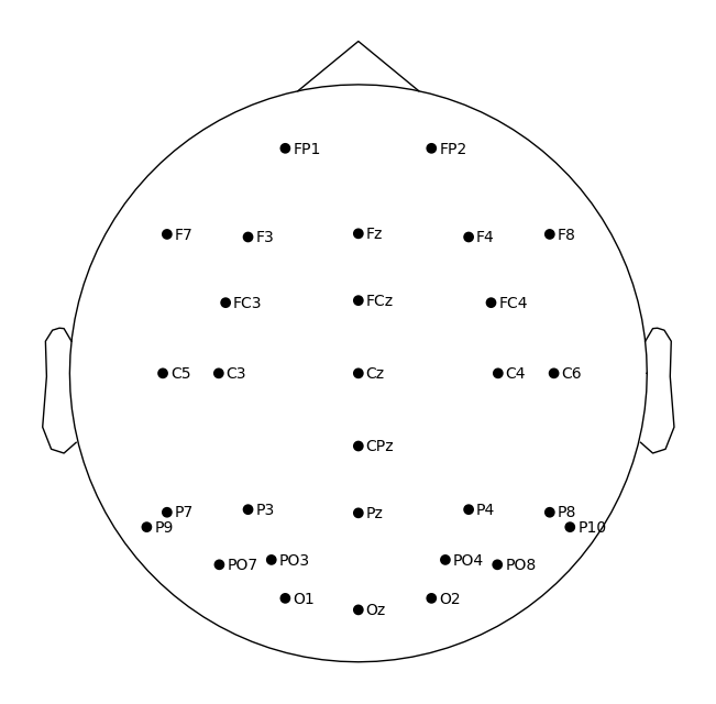
Then we load the locations of the EEG electrodes as provided by the manufacturer of the EEG system. Many of these standard EEG montages are shipped with MNE-Python.
raw = raw.set_montage('biosemi64', match_case=False)
_ = raw.plot_sensors(show_names=True)
2.6. Filter data#
Filtering is a common preprocessing step that is used to remove parts of the EEG signal that are unlikely to contain brain activity of interest. There are four different types of filters:
A high-pass filter removes low-frequency noise (e.g., slow drifts due to sweat or breathing)
A low-pass filter removes high-frequency noise (e.g., muscle activity)
A band-pass filter combines a high-pass and a low-pass filter
A band-stop filter removes a narrow band of frequencies (e.g., 50 Hz line noise)
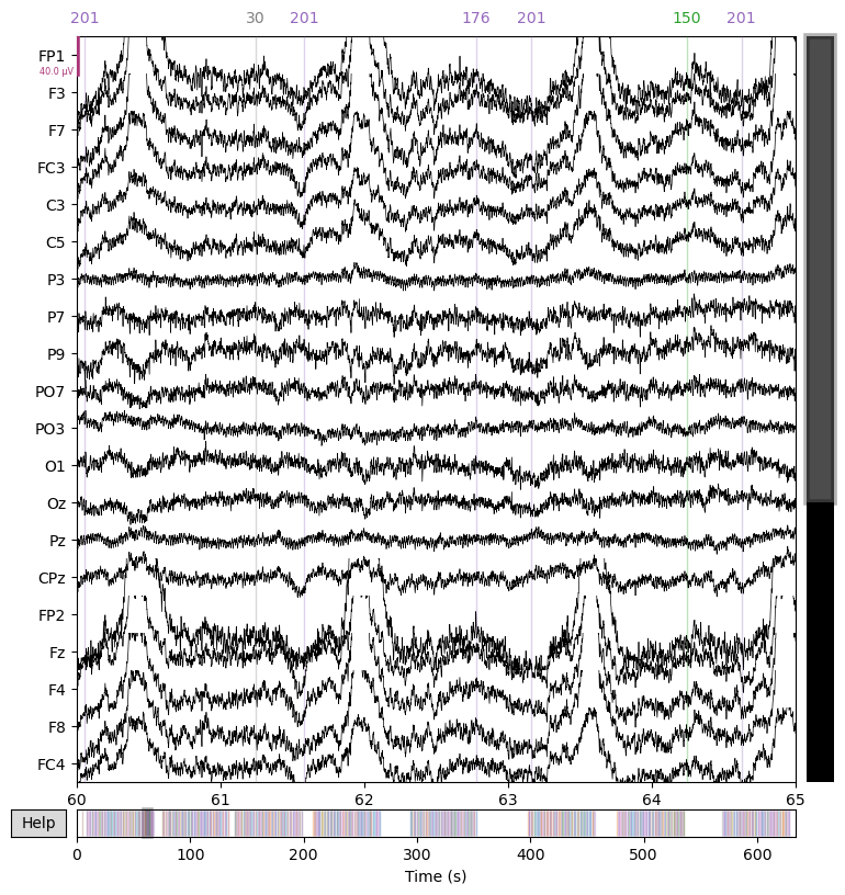
We first apply a high-pass filter at 0.1 Hz to remove slow drifts and plot the filtered data.
raw = raw.filter(l_freq=0.1, h_freq=None)
_ = raw.plot(start=60.0, duration=5.0)
Filtering raw data in 1 contiguous segment
Setting up high-pass filter at 0.1 Hz

FIR filter parameters
---------------------
Designing a one-pass, zero-phase, non-causal highpass filter:
- Windowed time-domain design (firwin) method
- Hamming window with 0.0194 passband ripple and 53 dB stopband attenuation
- Lower passband edge: 0.10
- Lower transition bandwidth: 0.10 Hz (-6 dB cutoff frequency: 0.05 Hz)
- Filter length: 33793 samples (33.001 s)
[Parallel(n_jobs=1)]: Done 17 tasks | elapsed: 0.4s
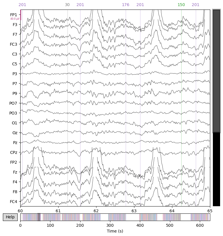
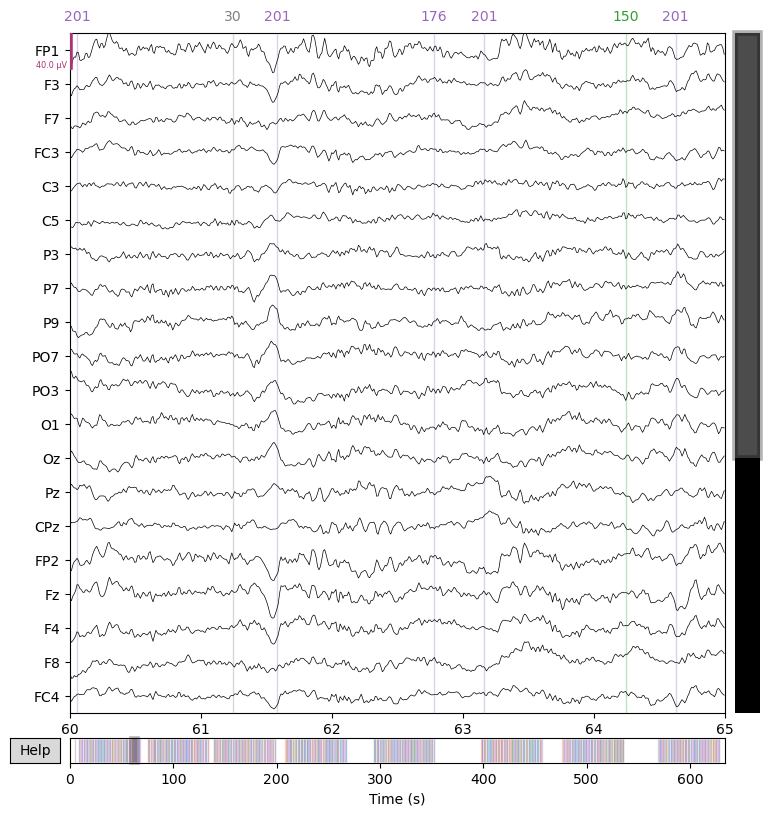
Next, we apply a low-pass filter at 30 Hz to remove high-frequency noise and plot the data again.
raw = raw.filter(l_freq=None, h_freq=30.0)
_ = raw.plot(start=60.0, duration=5.0)
Filtering raw data in 1 contiguous segment
Setting up low-pass filter at 30 Hz

FIR filter parameters
---------------------
Designing a one-pass, zero-phase, non-causal lowpass filter:
- Windowed time-domain design (firwin) method
- Hamming window with 0.0194 passband ripple and 53 dB stopband attenuation
- Upper passband edge: 30.00 Hz
- Upper transition bandwidth: 7.50 Hz (-6 dB cutoff frequency: 33.75 Hz)
- Filter length: 451 samples (0.440 s)
[Parallel(n_jobs=1)]: Done 17 tasks | elapsed: 0.2s
Note that we’ve performed these two filters separately for demonstration purposes, but we could have also applied a single band-pass filter.
2.7. Correct eye artifacts#
Eye blinks and eye movements are the most prominent source of artifacts in EEG data. They are approximately 10 times larger than the brain signals we are interested in and affect especially frontal electrodes.
There are multiple ways to remove eye artifacts from EEG data. The most common one is a machine learning technique called independent component analysis (ICA). ICA decomposes the EEG data into a set of independent components, each of which represents a different source of EEG activity.
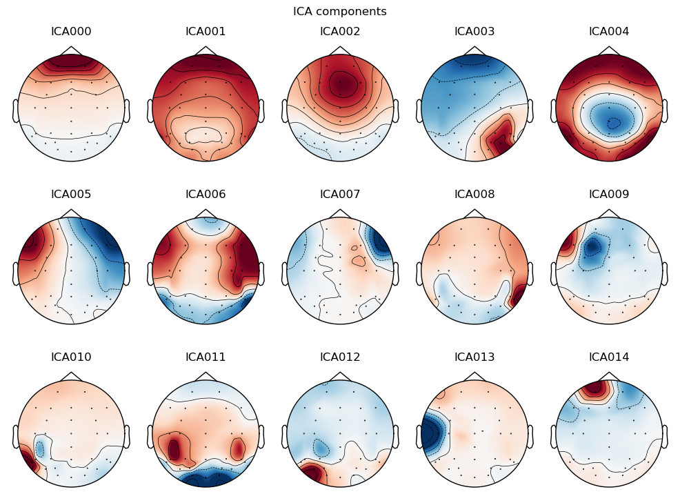
Each component is characterized by a topography (i.e., a spatial pattern of activity across electrodes) and a time course (i.e., a pattern of activity over time). We can use these to identify components that we think reflect eye artifacts, and remove them from the data.
ICA is typically computed based on a high-pass filtered copy of the data (cutoff = 1 Hz). We ask the algorithm to identify 15 components and plot their scalp topographies.
raw_copy = raw.copy().filter(l_freq=1.0, h_freq=None)
ica = ICA(n_components=15)
ica = ica.fit(raw_copy)
_ = ica.plot_components()
Filtering raw data in 1 contiguous segment
Setting up high-pass filter at 1 Hz

FIR filter parameters
---------------------
Designing a one-pass, zero-phase, non-causal highpass filter:
- Windowed time-domain design (firwin) method
- Hamming window with 0.0194 passband ripple and 53 dB stopband attenuation
- Lower passband edge: 1.00
- Lower transition bandwidth: 1.00 Hz (-6 dB cutoff frequency: 0.50 Hz)
- Filter length: 3381 samples (3.302 s)

Fitting ICA to data using 30 channels (please be patient, this may take a while)
Selecting by number: 15 components
Fitting ICA took 6.6s.
[Parallel(n_jobs=1)]: Done 17 tasks | elapsed: 0.2s
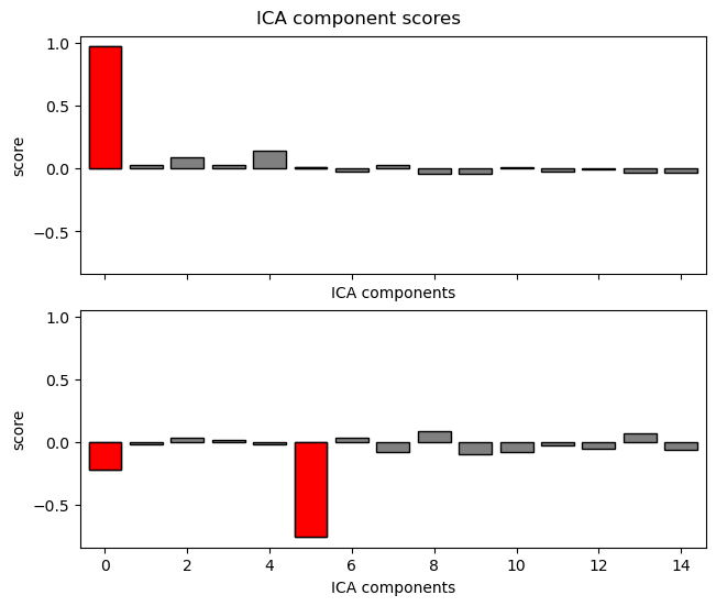
Then we can use a clever method that automatically identifies components that are likely to reflect eye artifacts (based on the correlation of the component’s time course with our two VEOG and HEOG channels).
eog_indices, eog_scores = ica.find_bads_eog(raw, ch_name=['HEOG', 'VEOG'],
                                            verbose=False)
ica.exclude = eog_indices
_ = ica.plot_scores(eog_scores)
/tmp/ipykernel_4300/1872092502.py:1: FutureWarning: The default for pick_channels will change from ordered=False to ordered=True in 1.5 and this will result in a change of behavior because the resulting channel order will not match. Either use a channel order that matches your instance or pass ordered=False.
  eog_indices, eog_scores = ica.find_bads_eog(raw, ch_name=['HEOG', 'VEOG'],
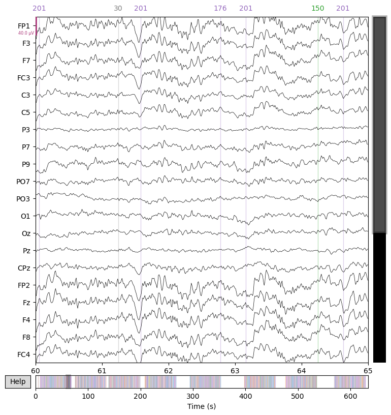
Finally, by “applying” the ICA to the data (formally, back-projecting the non-artifact components from component space to channel space), we can remove the eye artifacts from the data.
raw = ica.apply(raw)
_ = raw.plot(start=60.0, duration=5.0)
Applying ICA to Raw instance
    Transforming to ICA space (15 components)
    Zeroing out 2 ICA components
    Projecting back using 30 PCA components
2.8. Re-reference data#
Re-referencing is our final preprocessing step. Since the EEG signal is measured as the difference in voltage between two electrodes, the signal at any given electrode depends strongly on the “online” reference electrode (typically placed on the mastoid bone behind the ear or on the forehead).
During preprocessing (“offline”), we typically want to re-reference the data to a more neutral (and less noisy) reference, such as the average of all channels.
raw = raw.set_eeg_reference('average')
_ = raw.plot(start=60.0, duration=5.0)
EEG channel type selected for re-referencing
Applying average reference.
Applying a custom ('EEG',) reference.
2.9. Exercises#
Re-run the above analysis for a different experiment. For this, you can simply reuse the code cells above, changing only the second cell. Valid experiment names are
'N170','MMN','N2pc','N400','P3', or'ERN'.Below, try out the effect of different filter settings such as a higher high-pass cutoff or a lower low-pass cutoff. For this, write your own code that achieves the following: (a) read the raw data from one participant, (b) apply your own custom high-pass, low-pass, or band-pass filter, (c) plot the filtered data, and (d) repeat for different filter settings.
# Your code goes here
...
2.10. Further reading#
Tutorials on preprocessing on the MNE-Python website
Blog post Pitfalls of filtering the EEG signal by Narayan P. Subramaniyam
Blog post Introduction to ICA: Independent Component Analysis by Jonas Dieckmann
Online chapter A closer look at ICA-based artifact correction in Luck (2014)
Paper EEG is better left alone (Delorme, 2023)
2.11. References#
- Delorme, 2023
Delorme, A. (2023). EEG is better left alone. Scientific Reports, 13(1), 2372. doi:10.1038/s41598-023-27528-0
- Gramfort et al., 2013
Gramfort, A., Luessi, M., Larson, E., Engemann, D. A., Strohmeier, D., Brodbeck, C., … Hämäläinen, M. (2013). MEG and EEG data analysis with MNE-Python. Frontiers in Neuroscience, 7, 267. doi:10.3389/fnins.2013.00267
- Kappenman et al., 2021(1,2)
Kappenman, E. S., Farrens, J. L., Zhang, W., Stewart, A. X., & Luck, S. J. (2021). ERP CORE: An open resource for human event-related potential research. NeuroImage, 225, 117465. doi:10.1016/j.neuroimage.2020.117465
- Luck, 2014
Luck, S. J. (2014). An Introduction to the Event-Related Potential Technique. 2 ed. Cambridge, Massachusetts: MIT Press.