4. Averaging#
The EEG is a very noisy signal. Therefore, if we are interest in the brain’s response to a certain event (e.g., seeing a face versus a car), we need to average the EEG response over many trials (repetitions) of that event (i.e., over many different face trials and many different car trials). With this averaging procedure, unsystematic noise will get canceled out, while the systematic brain response will remain.
Averaging is performed separately for each EEG channel and timepoint, reducing the dimensionality of the data from trials × channels × timepoints (epochs) to channels × timepoints (average).
Fig. 4.1 Continuous, epoched, and averaged EEG. Source: Luck (2022)#
In “traditional” ERP analysis, these averages (separately for each participant and condition) are also used for statistical testing (using \(t\)-tests or ANOVAs), but modern approaches (e.g., linear mixed models) are typically performed on the single trials data (before averaging). Averaging remains useful for visualization purposes.
Goals
Creating an averaged ERP (“evoked”)
Plotting evokeds as time courses and topographies
4.1. Load Python packages#
As before, all the functions we’ll need are provided by the MNE-Python (Gramfort et al, 2013) and pandas packages.
# %pip install mne hu-neuro-pipeline pandas
import pandas as pd
from mne import Epochs, combine_evoked, merge_events, set_bipolar_reference
from mne.io import read_raw
from mne.preprocessing import ICA
from mne.viz import plot_compare_evokeds
from pipeline.datasets import get_erpcore
4.2. Recreate epochs#
We repeat the preprocessing and epoching steps from the previous chapters in a condensed form (without any intermediate plots).
Show code cell source
# Download data
files_dict = get_erpcore('N170', participants='sub-004', path='data')
raw_file = files_dict['raw_files'][0]
log_file = files_dict['log_files'][0]

# Preprocessing
raw = read_raw(raw_file, preload=True)
raw = set_bipolar_reference(raw, anode='FP1', cathode='VEOG_lower',
                            ch_name='VEOG', drop_refs=False)
raw = set_bipolar_reference(raw, anode='HEOG_right', cathode='HEOG_left',
                            ch_name='HEOG', drop_refs=False)
raw = raw.set_channel_types({'VEOG': 'eog', 'HEOG': 'eog'})
raw = raw.drop_channels(['VEOG_lower', 'HEOG_right', 'HEOG_left'])
raw = raw.set_montage('biosemi64', match_case=False)
raw = raw.filter(l_freq=0.1, h_freq=30.0)
raw_copy = raw.copy().filter(l_freq=1.0, h_freq=None, verbose=False)
ica = ICA(n_components=15)
ica = ica.fit(raw_copy)
eog_indices, eog_scores = ica.find_bads_eog(raw, ch_name=['VEOG', 'HEOG'],
                                            verbose=False)
ica.exclude = eog_indices
raw = ica.apply(raw)
raw = raw.set_eeg_reference('average')

# Epoching
log = pd.read_csv(log_file, sep='\t')
events = log[['sample', 'duration', 'value']].values.astype(int)
events = merge_events(events, ids=range(1, 41), new_id=1)
events = merge_events(events, ids=range(41, 81), new_id=2)
event_id = {'face': 1, 'car': 2}
epochs = Epochs(raw, events, event_id, tmin=-0.2, tmax=0.8,
                baseline=(-0.2, 0.0), preload=True)
epochs = epochs.drop_bad({'eeg': 100e-6})
Show code cell output
Reading /home/runner/work/intro-to-eeg/intro-to-eeg/ipynb/data/erpcore/N170/sub-004/eeg/sub-004_task-N170_eeg.fdt
Reading 0 ... 649215  =      0.000 ...   633.999 secs...
EEG channel type selected for re-referencing
Creating RawArray with float64 data, n_channels=1, n_times=649216
    Range : 0 ... 649215 =      0.000 ...   633.999 secs
Ready.
Added the following bipolar channels:
VEOG
EEG channel type selected for re-referencing
Creating RawArray with float64 data, n_channels=1, n_times=649216
    Range : 0 ... 649215 =      0.000 ...   633.999 secs
Ready.
Added the following bipolar channels:
HEOG
Filtering raw data in 1 contiguous segment
Setting up band-pass filter from 0.1 - 30 Hz

FIR filter parameters
---------------------
Designing a one-pass, zero-phase, non-causal bandpass filter:
- Windowed time-domain design (firwin) method
- Hamming window with 0.0194 passband ripple and 53 dB stopband attenuation
- Lower passband edge: 0.10
- Lower transition bandwidth: 0.10 Hz (-6 dB cutoff frequency: 0.05 Hz)
- Upper passband edge: 30.00 Hz
- Upper transition bandwidth: 7.50 Hz (-6 dB cutoff frequency: 33.75 Hz)
- Filter length: 33793 samples (33.001 s)

Fitting ICA to data using 30 channels (please be patient, this may take a while)
Selecting by number: 15 components
Fitting ICA took 8.5s.
Applying ICA to Raw instance
    Transforming to ICA space (15 components)
    Zeroing out 2 ICA components
    Projecting back using 30 PCA components
EEG channel type selected for re-referencing
Applying average reference.
Applying a custom ('EEG',) reference.
Not setting metadata
160 matching events found
Applying baseline correction (mode: mean)
0 projection items activated
Using data from preloaded Raw for 160 events and 1025 original time points ...
0 bad epochs dropped
    Rejecting  epoch based on EEG : ['F8']
    Rejecting  epoch based on EEG : ['F3', 'C5', 'P9', 'PO7', 'P10', 'PO8', 'O2']
    Rejecting  epoch based on EEG : ['P9', 'P10', 'PO8', 'O2']
    Rejecting  epoch based on EEG : ['F3', 'F4']
    Rejecting  epoch based on EEG : ['F8']
5 bad epochs dropped
[Parallel(n_jobs=1)]: Done 17 tasks | elapsed: 0.3s
This gives us the cleaned, epoched data as an Epochs object.
epochs
| Number of events | 155 |
|---|---|
| Events | car: 79 face: 76 |
| Time range | -0.200 – 0.800 s |
| Baseline | -0.200 – 0.000 s |
4.3. Averaging#
The actual averaging step is simple: We just need to use the average() method on an Epochs object.
This will return an Evoked object, which contains the averaged data (channels × timepoints).
evokeds = epochs.average()
evokeds
| Condition | 0.49 × face + 0.51 × car |
|---|---|
| Data kind | average |
| Timepoints | 1025 samples |
| Channels | 30 channels |
| Number of averaged epochs | 155 |
| Time range (secs) | -0.2001953125 – 0.7998046875 |
| Baseline (secs) | -0.200 – 0.000 s |
evokeds.get_data().shape
(30, 1025)
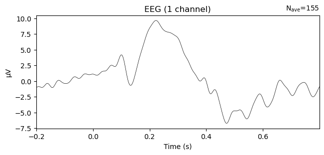
Like all MNE objects, evokeds have a plot() method to visualize the averaged time course at a single EEG channel:
_ = evokeds.plot(picks='PO8')
Need more than one channel to make topography for eeg. Disabling interactivity.
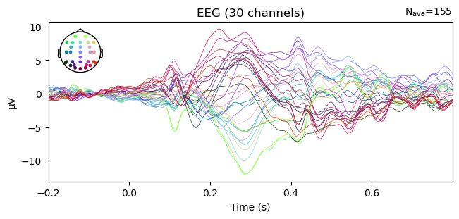
Or at all channels (also called a butterfly plot):
_ = evokeds.plot()
But wait!
Now we have averaged across all trials, but we are interested in the difference between face and car trials.
To do so, we can perform the averaging twice, each time selecting only the epochs of one of the two conditions.
We add a string as a comment to each evoked object to keep track of which is which.
evokeds_face = epochs['face'].average()
evokeds_face.comment = 'face'
evokeds_face
| Condition | face |
|---|---|
| Data kind | average |
| Timepoints | 1025 samples |
| Channels | 30 channels |
| Number of averaged epochs | 76 |
| Time range (secs) | -0.2001953125 – 0.7998046875 |
| Baseline (secs) | -0.200 – 0.000 s |
evokeds_car = epochs['car'].average()
evokeds_car.comment = 'car'
evokeds_car
| Condition | car |
|---|---|
| Data kind | average |
| Timepoints | 1025 samples |
| Channels | 30 channels |
| Number of averaged epochs | 79 |
| Time range (secs) | -0.2001953125 – 0.7998046875 |
| Baseline (secs) | -0.200 – 0.000 s |
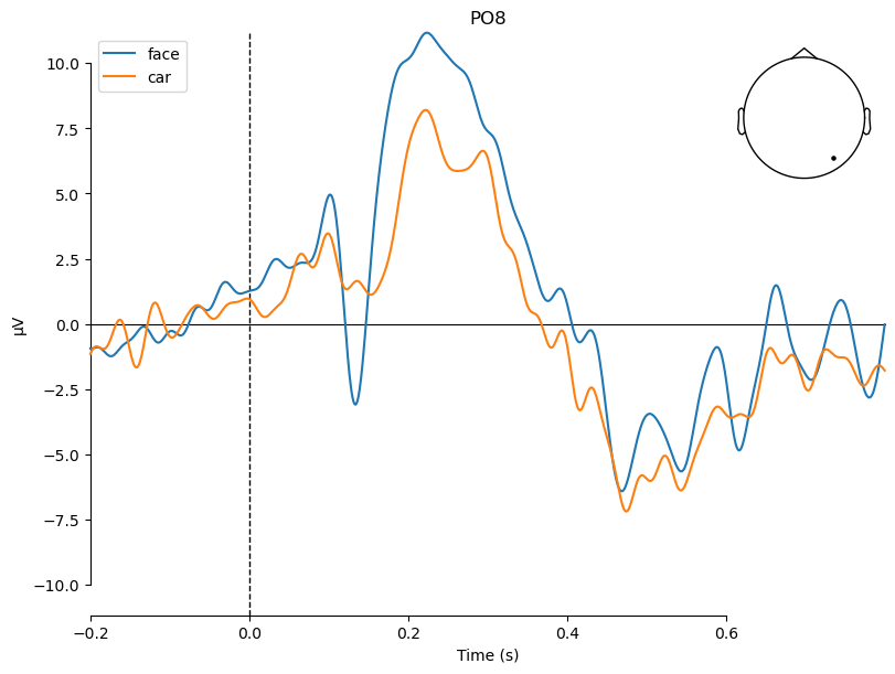
That way, we can now compare the two conditions by showing both of them in the same plot:
evokeds_list = [evokeds_face, evokeds_car]
_ = plot_compare_evokeds(evokeds_list, picks='PO8')
4.4. Difference wave#
From the two separate evokeds for the two conditions, we can also compute a difference wave, which is simply the difference (subtraction) between the two evokeds at each time point.
There are multiple ways to implement this subtraction in code.
One would be to extract the two Numpy arras (using the get_data() method) and then subtract them from one another.
Or we could use MNE’s combine_evoked() function with a specific set of weights that will perform the subtraction:
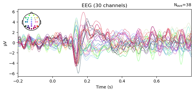
evokeds_diff = combine_evoked(evokeds_list, weights=[1, -1])
evokeds_diff.comment = 'face - car'
_ = evokeds_diff.plot()
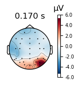
The time course plots that we have created thus far are showing the data for a single EEG channel and all time points (i.e., one row of the data matrix). Alternatively, we could plot the data for all EEG channels at a single time point (i.e., one column of the data matrix). This is called a scalp topography.
_ = evokeds_diff.plot_topomap(times=[0.17])
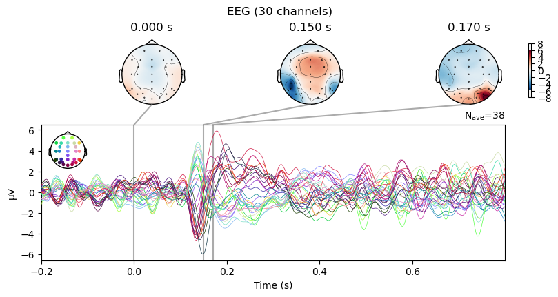
The Evoked object even has a method to plot the time course (butterfly) plot and a few scalp topographies at the same time:
_ = evokeds_diff.plot_joint(times=[0.0, 0.15, 0.17])
No projector specified for this dataset. Please consider the method self.add_proj.
4.5. Exercises#
Repeat the preprocessing and epoching (first code cell) for a different ERP CORE experiment (valid experiment names are
'N170','MMN','N2pc','N400','P3', or'ERN'). Create evokeds for the two conditions in your experiment and visualize them using time course and scalp topography plots.
# Your code goes here
...
4.6. Further reading#
Tutorial on evokeds on the MNE-Python website
4.7. References#
- Gramfort et al., 2013
Gramfort, A., Luessi, M., Larson, E., Engemann, D. A., Strohmeier, D., Brodbeck, C., … Hämäläinen, M. (2013). MEG and EEG data analysis with MNE-Python. Frontiers in Neuroscience, 7, 267. doi:10.3389/fnins.2013.00267
- Luck, 2022
Luck, S. J. (2022). A very brief introduction to EEG and ERPs. Applied Event-Related Potential Data Analysis. LibreTexts. https://doi.org/10.18115/D5QG92.